Process Mining Performance: Benchmarks and Tips

What Drives Process Mining Performance

Process mining performance depends on three factors: how much data you upload, how you structure it, and how the system processes it. This guide covers all three with real benchmarks and practical ways to improve results.

We publish all our numbers. Compare them with any process mining tool on the market.

The Data Pipeline: Where Time Goes

When you upload data to ProcessMind, three things happen. Here’s exactly where the time goes:

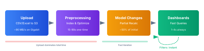
1. Upload (dominates total time). Your file travels over the internet to our cloud infrastructure. This is the bottleneck for large files. Physics wins: a 50 million event CSV (11 GB) takes 2 minutes on gigabit, 18 minutes on 100 Mbps, or over 3 hours on 10 Mbps. The same data in Parquet is just 1.7 GB, cutting those times to 19 seconds, 3 minutes, and 28 minutes. This is the primary reason to use columnar formats like Parquet or ORC, or smaller datasets.

2. Preprocessing (one-time cost, ~30s to 2.5 min). Once uploaded, we transform your data into optimized columnar storage: events indexed, activity transitions pre-computed, process variants identified, and summary statistics calculated. This takes 30 seconds for small datasets and up to 2.5 minutes for 100M events. You pay this cost once per upload and benefit from it thereafter.

3. Model changes (partial recalculation, 6–52s). When you modify the process model by adding or removing activities or changing mappings, only the model-dependent calculations are updated. This takes 6 seconds for small datasets and up to 52 seconds for 100M events, much faster than full preprocessing. Filter changes are instant.

Understanding Query Performance

Once your data is loaded, several characteristics determine query speed. Understanding them helps you design better exports and set realistic expectations.

Activity count matters. Process models with 10–20 distinct activities are optimal. Above 50 activities, the process flow takes longer to compute and becomes harder to understand. Too many nodes and edges create visual noise. If your export contains many activities, consider grouping related steps.

Variant diversity affects computation. A process where 80% of cases follow 5 variants is faster to analyze than one where every case takes a unique path. High variation isn’t bad and often signals real problems, but expect slightly longer query times.

More columns means more scanning. Each attribute you include is indexed and queried. The core columns, CaseId, Activity, and Timestamp, are always needed. Additional columns help with filtering and categorization, but each adds overhead.

Long cases take longer. A case with 50 events requires more computation than one with 5. If your process has cases spanning hundreds of events, queries will be proportionally slower. This is inherent to process mining, not specific to any tool.

Real-World Benchmark Data (March 2026)

Understanding what to expect helps you plan. These benchmarks run on production AWS infrastructure with real network latency and are averaged across multiple test runs. We tested 50+ query types per dataset size.

Upload and Preprocessing Times

The table below shows realistic expectations for each dataset size. Upload time dominates for larger files, especially on slower connections. It is the single biggest factor in your total wait time.

File sizes are for uncompressed CSV with a typical event log schema (CaseId, Activity, Timestamp, plus 5–8 business attributes). Your files may be larger or smaller depending on column count and content.

1 Gbps upload times are measured, with 88 MB/s effective throughput to AWS eu-central-1. Other speeds are extrapolated at practical throughputs: 50 Mbps → ~5 MB/s, 100 Mbps → ~10 MB/s, 10 Mbps → ~1 MB/s. Real-world throughput depends on your network, distance to the data center, and current load.

The key insight: Preprocessing time plateaus between 1 and 2.5 minutes regardless of scale. Upload time scales linearly with file size. Reducing file size is the highest-leverage optimization you can make.

Choose the Right File Format

The file format you upload has a major impact on upload speed and preprocessing time. ProcessMind supports CSV, Parquet, ORC, Excel, and XES. For large datasets, Parquet and ORC dramatically outperform CSV in both file size and processing speed.

File Size Comparison

Parquet files are 85% smaller than CSV. ORC files are 82% smaller. Both are columnar formats with built-in compression, so no extra step is required. Your ETL tool or data platform, such as Spark, Databricks, dbt, or BigQuery, likely already supports exporting to Parquet or ORC.

Preprocessing by Format

File size is only half the story. After upload, your data goes through format-dependent ingestion and analytics computation, including event indexing and transition and variant calculations. The analytics step dominates and is the same for all formats. CSV.GZ is the only format that adds significant extra time because gzip files cannot be split for parallel decompression.

Preprocessing time is nearly identical for Parquet, ORC, and CSV because analytics computation dominates regardless of input format. But CSV.GZ preprocessing degrades significantly at scale, growing from about a minute at 1M events to over 4 minutes at 100M. Gzip-compressed files cannot be split and processed in parallel, so decompression adds a growing step before analytics can begin.

The Total Picture

Consider both upload time and preprocessing, and the format choice becomes clear:

At scale, Parquet and ORC are the clear winners because their file sizes are dramatically smaller. Upload time is the main bottleneck. Preprocessing takes roughly the same time for all formats except CSV.GZ, which incurs a growing decompression penalty.

Delta Loading: Add Data Without Re-uploading

Once you have loaded a baseline dataset, you don’t need to re-upload everything when new data arrives. ProcessMind supports delta loading, or incremental uploads, so you can append new events to an existing dataset.

How it works:

1. Upload your initial dataset, such as Q1 2026 purchase orders with 2.3M events
2. When Q2 data arrives, upload only the new events as a delta file, such as 800K new events
3. ProcessMind merges the files automatically and reprocesses

The performance impact is significant. Instead of re-uploading your growing dataset each time, you upload only what’s new:

After a delta upload, preprocessing runs again on the combined dataset, with the same 1–2.5 min cost. But you save all the upload time for data you already uploaded.

Delta loading is ideal for:

• Weekly or monthly data refreshes: append new transactions as they become available
• Continuous process monitoring: keep dashboards current without large uploads
• Growing event logs: add new events from ERP, CRM, or other source systems

Delta files must use the same file format and column structure as the original upload. See the incremental data loading guide for details.

Using the API for Large or Automated Uploads

For datasets exceeding a few gigabytes or recurring uploads, scripts or command-line tools are more reliable than browser uploads. Browsers can time out, consume excessive memory, or lose progress when the network is interrupted.

Why the API works better for large files:

• Reliable transfers. If your connection drops, you can retry without starting over.
• No browser memory limits. Browsers struggle with multi-gigabyte files. Command-line tools handle them easily.
• Automation. Schedule nightly uploads, integrate with ETL pipelines, or trigger uploads from CI/CD.
• Progress monitoring. Tools like curl show real-time transfer progress.
• Delta uploads. Programmatically append new data on a schedule.

Example using curl:

# Upload a Parquet file directly using a presigned URL
curl -X PUT "$PRESIGNED_URL" --upload-file data.parquet

ProcessMind provides presigned URLs that authorize direct uploads to cloud storage. No credentials beyond your API key are required. You can also copy the presigned upload URL directly from the dataset settings menu in the ProcessMind UI.

See the API documentation for complete Bash, JavaScript, and Python examples, including how to obtain presigned URLs, upload delta files, and handle large datasets programmatically.

Model Iteration Speed

When you refine your process model by renaming activities, changing mappings, or adding groupings, only the model-dependent calculations need updating. The base data stays in place:

Model changes are fast because the initial data loading step, which grows with dataset size, is already complete. Only the model-dependent aggregation step, including activity mappings, transitions, and variants, runs again. For datasets up to 20M events, model changes complete in under 25 seconds. Even at 100M events, they take under a minute, much faster than full preprocessing.

Dashboard Response Times

Once your data is loaded, these are the response times you experience during analysis. The times below are medians across multiple benchmark runs. Each dashboard component queries independently and loads in parallel:

Patterns to notice:

• Statistics, including summary counts and durations, stay at ~0.6s regardless of size. These queries are highly optimized.
• Process Flow, the process diagram, scales with dataset size because it computes transitions between all activities.
• Variants and Categories scale moderately. Pre-aggregated data keeps them fast.
• Data Browser stays fast through pagination. With filters applied, it drops below 1s.
• Animation varies with the number of active cases being visualized.

The takeaway: At recommended dataset sizes of 1–10M events, every dashboard component responds in under 3.5 seconds. Even at 50M, most queries return in 2–4 seconds with filters applied. Only unfiltered process flows and category views on 50M+ datasets reach 5–6 seconds.

Start Small, Grow Big

This is the most important advice in this guide: don’t start with your largest dataset.

The numbers speak for themselves:

Most organizations find 1–5M events is more than enough for actionable insights. Process behavior stabilizes well before 10M events. Beyond that, you’re mostly adding duplicates of patterns you’ve already seen.

If your 1M event Parquet file, 34 MB, uploads in 3 seconds and gives you the same process map as 50M events, why wait 18 minutes?

Data Strategy: Finding the Right Size

The numbers above tell a clear story: at 1–5M events, uploads take seconds, preprocessing takes under 2 minutes, and dashboards respond in 1–2.5 seconds. At 50M, you’re waiting 20 minutes for an upload on 100 Mbps, and dashboards slow to 3–6 seconds. The experience is dramatically different.

So the real question isn’t “how fast is the tool?” It’s “how much data do I actually need?” The answer is almost always less than you think.

Segment First, Aggregate Later

Analyze one country, one department, or one product line first.

This isn’t about limitation. It’s about clarity. Segmented analysis produces sharper insights than global averages.

Why segmentation works:

• Processes differ by region. German operations follow different approval chains than US operations. French labor laws create different HR workflows. Analyzing them together creates noise.
• Different stakeholders, different priorities. The VP of EMEA cares about EMEA. Show them EMEA data. The global view can come later.
• Faster iteration. A single country’s data might be 500K events instead of 10M. You iterate in minutes, not hours.
• Built-in benchmarking. Once you’ve analyzed Germany, do the same for France. Now you can compare.

Example: A European logistics company with 42M shipment events across 8 countries:

• Analyzing everything: 42M events, 9.3 GB, 16 min upload (100 Mbps), 2 min preprocessing
• Analyzing Germany only: 8.5M events, 1.9 GB, 3 min upload, 1.5 min preprocessing
• Analyzing Netherlands only: 3.1M events, 690 MB, 1 min upload, 1 min preprocessing
• Using delta loading: upload Germany first, then append Netherlands when ready

Filter Out the Happy Path

Exclude the happy path before uploading. This technique can reduce datasets by 90–95%.

Most business processes follow the 80/20 rule. The vast majority of cases follow the standard, successful path. If you’re looking for exceptions, compliance violations, or process deviations, you don’t need that data.

Example: A purchase-to-pay process with 1.2 million purchase orders (8.4M events):

• 1.1M orders (92%) follow the happy path: Create PO → Approve → Goods Receipt → Invoice → Payment
• 96,000 orders (8%) have exceptions: rejections, returns, duplicate invoices, and missing approvals

If you’re analyzing compliance issues, export only the exception cases. That’s a 92% reduction, from 8.4M events (1.9 GB) to 670K events (150 MB). Upload time drops from 3 minutes to 15 seconds on 100 Mbps. Export as Parquet (15 MB), and you can upload it in under 2 seconds.

Column Selection: Less Is More

Every column you export costs bandwidth, storage, and processing time. Choosing columns carefully is one of the highest-impact optimizations you can make.

What to leave out:

• Long text fields. Order descriptions, comments, notes, and free-text fields. A 500-character description field across 5M events adds 2.5 GB to your file.
• PII (Personally Identifiable Information). Names, email addresses, and phone numbers. Removing PII reduces file size, eliminates privacy risks, and simplifies compliance.
• Redundant identifiers. If you have OrderId, you don’t need OrderGUID, OrderReference, or LegacyOrderNumber.
• Audit columns. CreatedBy, ModifiedBy, CreatedDate, and ModifiedDate. Unless you’re specifically analyzing them, leave them out.
• System columns. Internal flags, partition keys, and technical metadata.

Example: An SAP export of 1.8M purchase order events with 45 columns reduced to 12 essential columns:

• File size: 2.1 GB → 380 MB (82% reduction)
• As Parquet: 380 MB → 58 MB (another 85% reduction)
• Upload time (100 Mbps): 3.5 min → 6 seconds
• Same analytical value

The columns that matter: CaseId, Activity, Timestamp, and a few business attributes, such as status, amount, category, and region. Everything else is probably noise.

When Scale Matters

Some analytical questions genuinely require large datasets. Understanding when helps you make the right call:

• Rare event detection. Finding edge cases that occur 1 in 100,000 times requires a population large enough to contain meaningful samples. If you need to analyze 50 instances of a rare exception and it occurs 0.01% of the time, you need 500K cases.
• Low-frequency path measurement. Process variants that occur 0.1% of the time might be invisible in a 1M event sample but significant in a 50M event population.
• Compliance and audit. Some regulations require complete population coverage. Sampling isn’t acceptable.
• Multi-year trend analysis. Comparing Q1 2024 to Q1 2025 to Q1 2026 requires data spanning all three periods. Use delta loading to build this incrementally.

If you need 50M+ events, plan for it: use Parquet format, which reduces 11 GB CSV to 1.7 GB and speeds up preprocessing; use the API for reliable transfers; and use a fast network connection if available. After that first load, dashboards remain fast.

Keeping the Model and the Interface Fast

The sections above are about data volume. The other half of responsiveness comes from how the model and the dashboards are built:

• Simplify the model. Break large processes into modular subprocesses; a canvas with a thousand visible elements is slow to render and impossible to read. Run auto-layout after structural changes.
• Be selective with dashboards. Every chart and tile has to be calculated. Keep the charts someone acts on and move the rest to their own dashboard instead of stacking everything into one view.
• Match the chart to the dataset. On large datasets, avoid the visualizations that carry the most overhead (detailed pie charts, many-category breakdowns) in favor of charts that summarize.
• Apply filters with restraint. Filters are cheap individually and expensive in combination. Keep the set that answers your question, and remove it afterwards.
• Watch the animation. Animation cost grows with the number of active cases. Lower the speed, or switch off tails and effects, when you only need the flow — see Process Animation.
• Archive and revisit. Move old datasets and processes out of the active workspace, and use simulation with the time metrics to find the bottlenecks worth fixing instead of optimizing everything at once.

Next Steps

The best way to understand process mining performance is to experience it with your own data.

1. Start with a sample. Export 1M events from a recent time period in Parquet format. Upload them. Build your first model. See how quickly you can iterate.

2. Apply the techniques from this guide. Use columnar formats. Filter for exceptions. Segment by region. Remove unnecessary columns. Each optimization builds on the last.

3. Scale deliberately. Once you understand your process with 1M events, decide whether you need more. Usually, you don’t. When you do, use delta loading to append data instead of re-uploading it.

Start a free trial and see these benchmarks in action. For help sizing your dataset or optimizing your exports, contact us. We’ve helped hundreds of organizations find the right balance between data volume and analysis speed.